Digitization System for Film Negatives and Slides (II)

The last post, Digitization System for Film Negatives and Slides (I), was dedicated to comment the oportunity to use a former photographic enlarger head as a part of a film digitization system by means of a digital camera. This second post comments aspects related with the illumination eveness in the diffusser supporting the negatives or slides to be reproduced.

In first place it is necessary to check the lighting uniformity taking an image from the diffuser deliberately defocused. This defocusing helps to avoid material irregularities and possible dust particles on the diffuser surface. Plastic materials tend to charge static electricity and attract any kind of small particles. Defocusing the diffuser is also achieved the manner of its normal function when the focus is adjusted over the negative or slide surface. Provided that the originals to reproduce are completely flat, depth of field is not necessary and then the diaphragm aperture can be adjusted in order to avoid any problem with diffraction. This image must be taken with the camera, lens and aperture that will be used in the film digitization. It must also be taken into account the working distance for the film size. In the examples that follow, the camera and lens used corresponds with those described in the former post. The working lens aperture is f/11 and de negative carrier framed is of 4×5” (10×12.5cm).

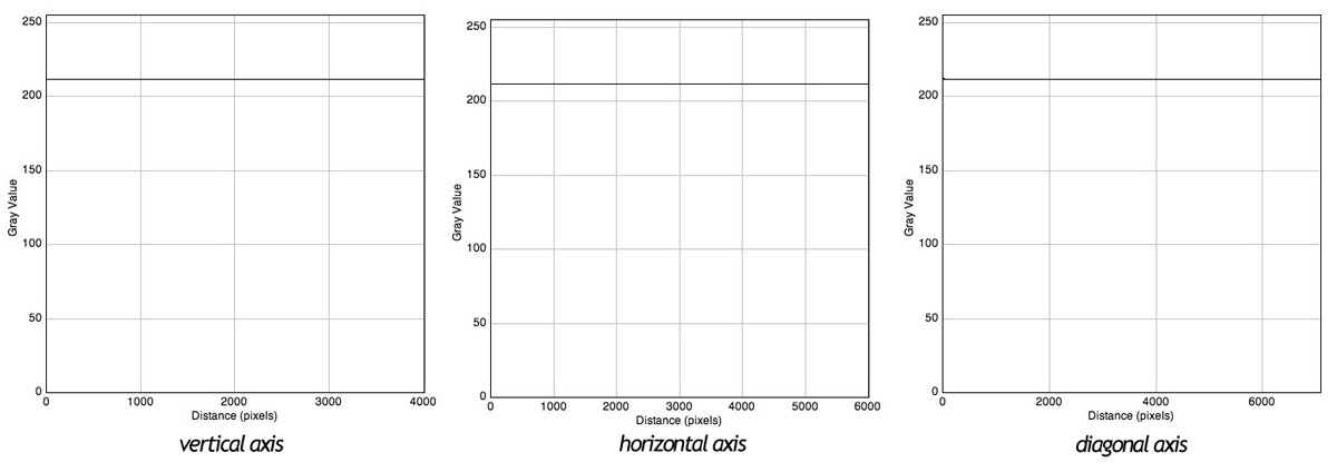
Once the diffuser image is available, it must be saved as a TIFF image format without compression in order to avoid changes in the pixel gray values. Next step is to take measurements of pixel brightness of at least three directions: Vertical axis, horizontal axis and diagonal axis. This can be done using several digital image processing software as ImageJ, NIHImage or Fiji. The Fig., 1 shows pixel gray value plots for those three axis in the case of the example.

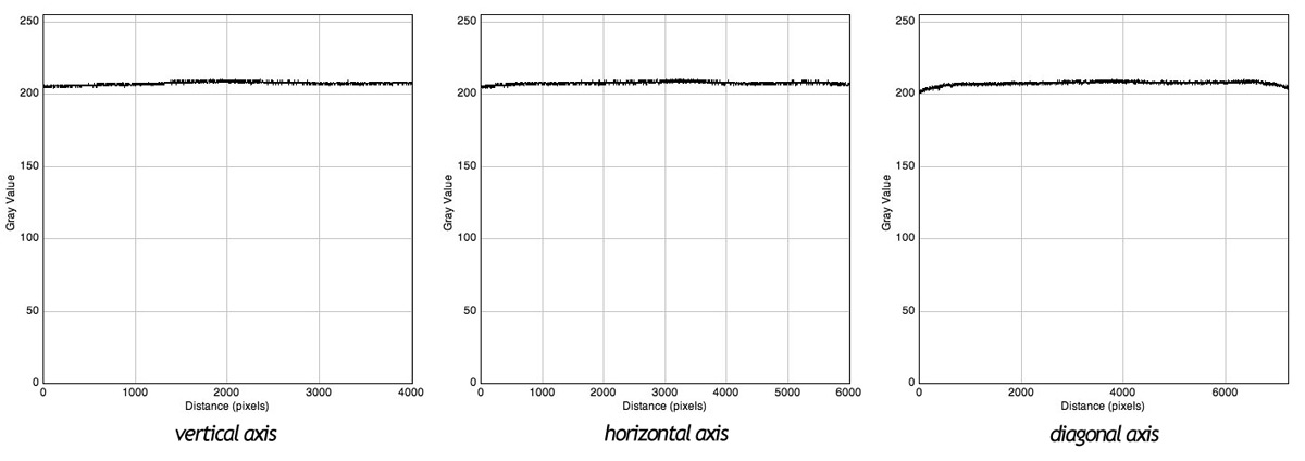
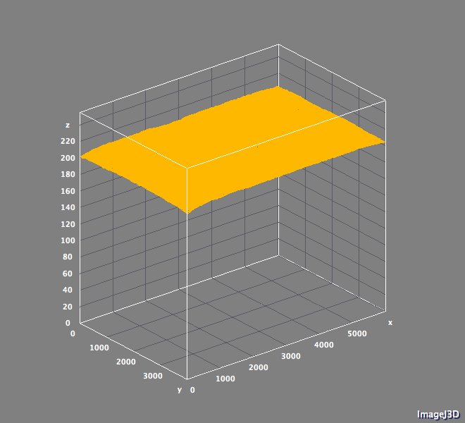
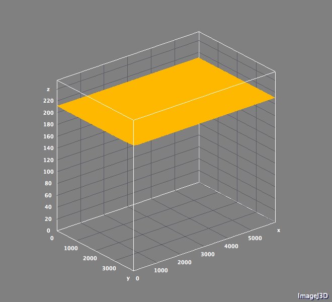
As can be observed, the illumination uniformity is near perfect with the system described. The differences between centre and corners are of less than ten gray values in the scale from 0 to 255 for the diagonal axis measurement. In the Fig., 2, a three dimensional graph of the whole image gray values, can be easily observed this little difference between. For the majority of applications, this little difference is absolutely negligible and hard to be detected by the naked eye, specially with pictorial images. In this case, the enlarger diffuser and the optical vignetting of the lens employed, match a high degree of performance for a correct reproduction. This series of assessment must be performed for all different taking distances suitable to frame the different film formats.

For those situations where the reproduction exigences a perfect degree of uniformity, that follows is a series of digital image processing that can be performed in order to compensate those little detected differences. The procedure allows to work in the defocused diffuser image into a software like Adobe Photoshop. The goal is to generate a Curves Adjustment Layer compensating those differences in luminosity.

The steps are as follow:

• First step is to take Color Samples in the center and the four corners of the image. Photoshop shows the results of the color samples in the Info Palette.
• Create a Curves Adjustment Layer on top of the Background Layer containing the defocused diffuser image.
• Copy to the System Clipboard the image on the Background Layer.
• Paste the previous copied image into the Curves Adjustment Layer Mask.
• Having selected this Layer Mask, invert the image values (Image>Adjustements>Invert).
• Selecting and viewing in the screen this Layer Mask (Option or Alt key + Click on the Layer Mask), apply a histogram expansion by means of the tool Levels or Curves. On both cases, the triangle sliders at left and right must be moved to the extremes of the histogram. Using the Levels tool, it is very important do not change manually the position of the gray triangle slider that indicates the middle value of the scale. In the case of the Curves tool, do not apply any change in shape other than the right line, now with a higher slope.
• Then, with the Layer Mask adjusted as previously described, modify the curve rising the brightness without any change in contrast. This is done modifying the Input and Output values of both Black and White in a such manner that the final shape is right and parallel to the previous default line. The values to apply will depend on the differences detected in the previous measurements.
• In any case, the effect caused by successive adjustments can be monitored by the indications in the Info Palette. Photoshop, being an active Adjustment Layer, indicates the gray value of the five color samples followed by the value they will take applying the corresponding adjustment. Each couple of values is separated by a slanted bar. The final “curve” shape must be a right line and parallel to the initial default right line.

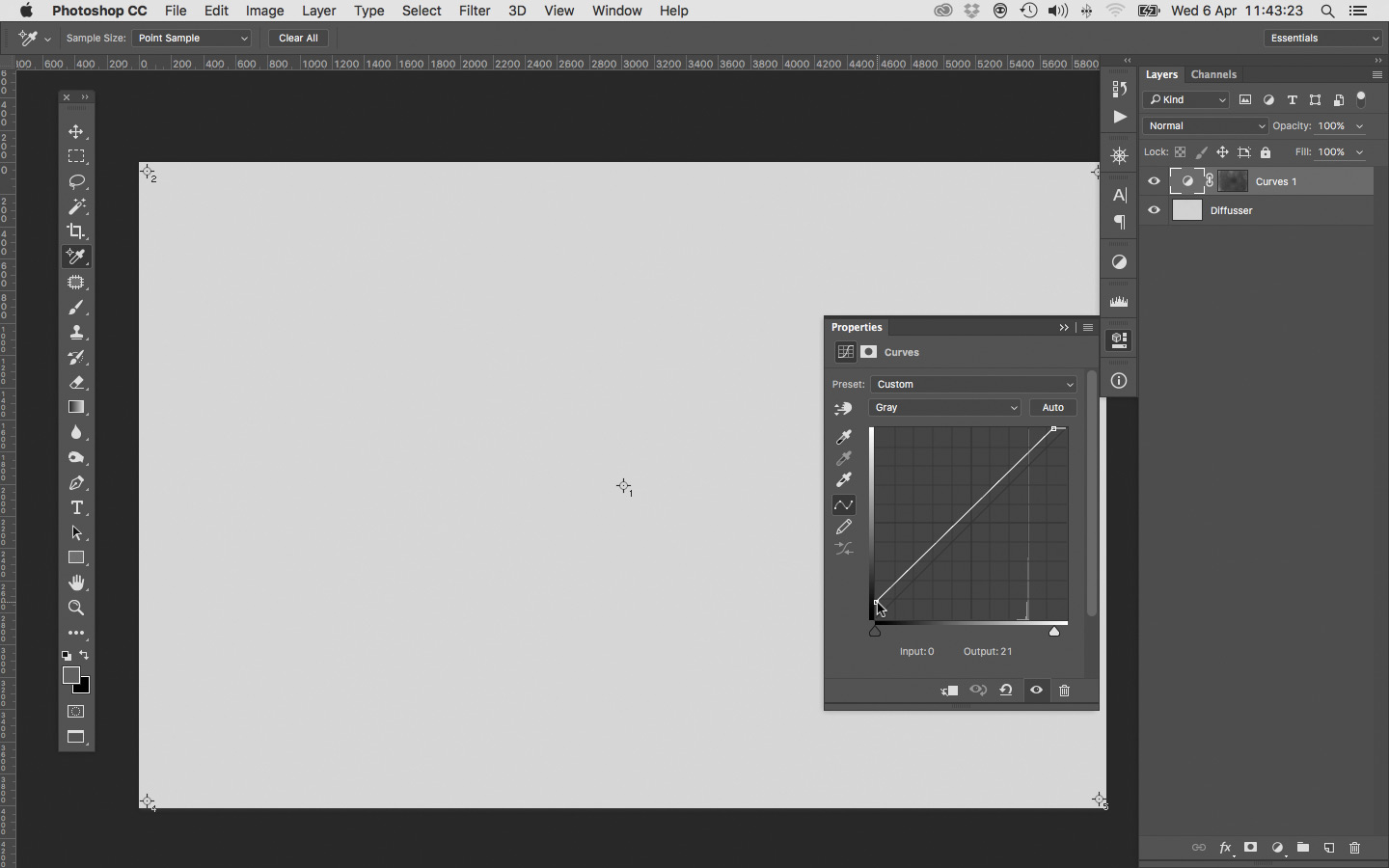
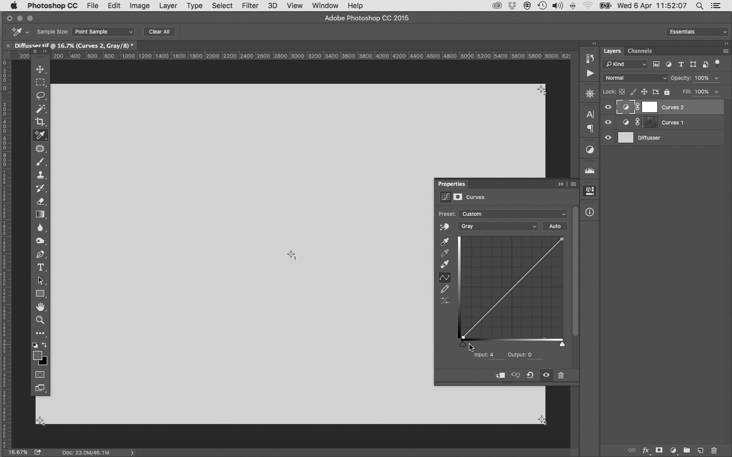
Remember that we are applying a uniform rising of luminosity that in turn is controlled by the contents of the Layer Mask. This mask contains all the image irregularities normalized to the scale from 0 to 255 and with its values inverted. The more dark the pixels in the mask, the lower the adjustment is applied to the image. Conversely, the lighter pixels in the mask represent the pixels of the image that will be modified. The adjustment will be complete in the areas where the mask pixels are plain white. The Fig., 3 shows the graphic interface from Adobe Photoshop with the curve applied in the example.

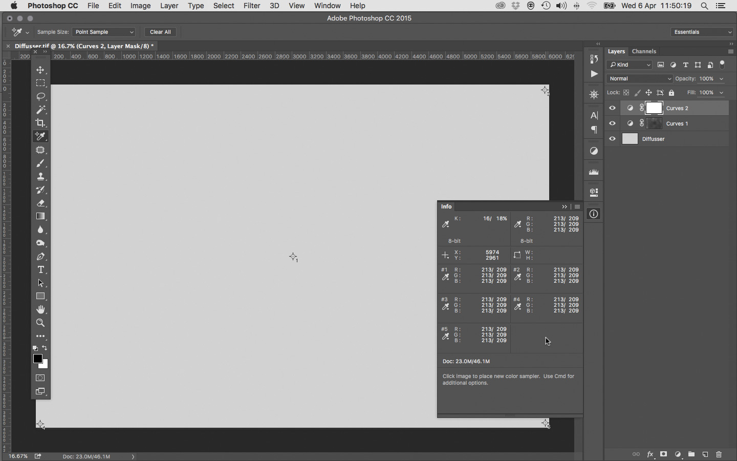
In the Info Palette shown at the Fig., 4 can be observed the gray values of the color samples before and after the curve adjustment. The example shows as after the curve adjustment, the values are the same for the center and the four corners of the image.

Nevertheless, the initial value in the center has raised four gray values into the scale from 0 to 255. Now we can follow fine tuning the curve adjustment or, even more simple, apply a second adjustment curve that diminishes those four gray values. Fig., 5 and 6 show this last correction.

These curves can be saved as custom pre-sets and then be applied on all the captures performed with the same working conditions. It can be also generated a Photoshop Action to be automaticly applied to a series of images laying in the same directory. Finally, the Fig., 7 and 8 show gray value plots similar to those previously shown (Fig., 1 and 2), after the smoothing of the illumination irregularities. All this plots confirm the efficiency of the proposed method.